
Fastest ecFFT in the West
Halo 2 builds its Lagrange-basis commitment key with an inverse FFT over elliptic-curve points. We improved its performance significantly.
Before a wallet can prove a transaction or cast a private vote, it must generate a proving key for the relevant circuit. When we profiled Zcash proof creation, that setup landed surprisingly near the top of the profile: on representative workloads, roughly 30% of the total time to build the key and create the proof.
Until recently, this cost would be paid on every transaction. We noticed this shortly before Ironwood and helped fix it; now, this setup is only executed on the first transaction after the wallet restarts. Even so, it remains a source of UX friction.
We have made Orchard ProvingKey::build 10× faster on Apple hardware, and are still working on it. A large gain came from a step that is not circuit-specific: before generating the circuit keys, ProvingKey::build constructs Halo 2's polynomial-commitment parameters, and constructing them takes an inverse FFT whose values are elliptic-curve points. We first made its scalar multiplications cheaper and then chose a dynamic FFT strategy that needs fewer of them.
The Lagrange-basis commitment key
The reason Halo 2 performs this transform starts with PLONK. A PLONK circuit is arranged as rows over a roots-of-unity domain

where  is a primitive
  th root of unity, and a circuit column containing the values
  is represented by a polynomial
  satisfying
  . Gate constraints, permutation arguments, and Halo 2's other polynomial relations are all built around values at these rows, so many of the polynomials that Halo 2 needs to commit to are represented by their evaluations over
  rather than by their monomial coefficients.
Halo 2's polynomial commitment scheme, however, starts from the monomial basis. It uses a vector of curve points  , and a polynomial

has the commitment

We could inverse-FFT every circuit column from its evaluation representation into monomial coefficients before committing to it, but we need to make these commitments repeatedly. Halo 2 instead does the basis conversion once, on the proving key itself. For the domain , define the Lagrange basis polynomials by

Any polynomial represented by its evaluations  can be written as

and because the commitment is linear, precomputing

lets us commit directly to the evaluation vector:

The obvious way to produce the  would be to construct each
  in the monomial basis and commit to it individually, but every Lagrange polynomial is dense, so this costs roughly scalar multiplications for each of basis polynomials:
  work. All of these polynomials are related, though. The coefficients of are

and therefore

In other words, the complete vector of Lagrange-basis generators is an inverse Fourier transform of the monomial-basis generators.
Because the transform is linear, we can apply it to the curve points themselves and compute all of the commitments at once.
An interesting property is that the entries of an FFT do not have to be field elements. They can be elements of an additive group. We just have to be able to add points and multiply them by field elements. Since is a power of two and the scalar field contains the required roots of unity, an inverse FFT over the curve points produces the whole vector of Lagrange generators in  operations rather than scalar multiplications.
What changes is the cost model. In a normal FFT, multiplying by a twiddle factor costs one field multiplication; here a nontrivial twiddle is a variable-base scalar multiplication requiring many curve additions and field operations. That is the curve FFT we wanted to optimize.
Radix-2 Cooley–Tukey
The standard implementation used the radix-2 Cooley–Tukey algorithm. Its central observation is that any polynomial can be split into its even- and odd-indexed coefficients,

and that the roots of unity come in opposite pairs: since

squaring either member of a pair gives the same argument,

So the half-size polynomials  and
and  only need to be evaluated once at
  , and the sign of the odd half is the only thing that changes between the two outputs:

Recursively repeating this split turns one size- transform into two size- transforms. In our transform the coefficients are curve points, so the bracketed factor is a scalar multiplication. The combine step is the familiar butterfly; in the implementation it appears layer by layer, after a bit-reversal permutation:

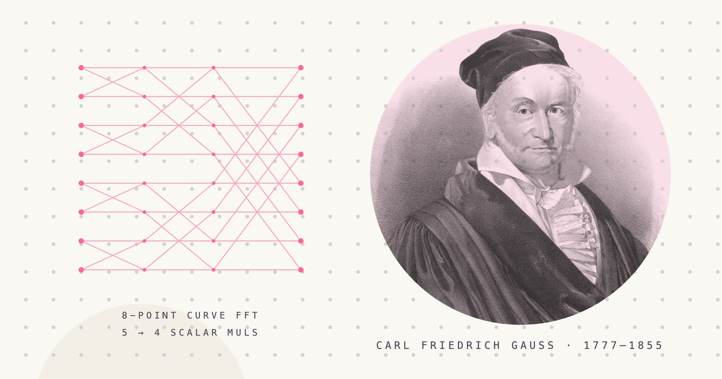
where  is the layer's twiddle factor. The first twiddle in every block is one and costs no scalar multiplication. All the other twiddles do. For an eight-point curve FFT, the radix-2 network has this cost:
| layer | blocks | nontrivial twiddles per block | scalar multiplications |
|---|---|---|---|
| 2-point | 4 | 0 | 0 |
| 4-point | 2 | 1 | 2 |
| 8-point | 1 | 3 | 3 |
| total | 5 |
Cooley–Tukey already replaced a quadratic transform with an one, but it optimizes its operation count under a much flatter cost model than ours, and it does not promise the fewest scalar multiplications for a small fixed transform in which multiplication is far more expensive than addition.
So the simple Cooley–Tukey FFT before we began our work had us at 9,217 scalar multiplications and 22,528 additions. We'd compute each scalar multiplication with 510 curve operations, taking us to a total cost of 4.72 million projective curve operations. In total: 54.4 million field multiply/square operations.
Cheaper scalar multiplications
Pallas and Vesta have a cheap order-three endomorphism  , and GLV decomposes a twiddle into two roughly half-size components,

where  is the order of the scalar field and
  is the scalar that acts by, so that

Our Eisenstein recoding and batch affine ladder work turns that decomposition into a short joint schedule, and the curve FFT is unusually friendly to it. The twiddles are public, and the same ones repeat across every block in a layer, so each distinct twiddle is decomposed once and all of the points it multiplies run through one batch of ladders in lockstep.
Keeping the FFT state in affine coordinates makes the batching pay twice. Affine addition needs a field inversion, which is expensive alone but cheap in bulk, and the ladders and the butterflies share the same batched inversions; the two butterfly outputs  and
and  share a single denominator.
This made the conventional radix-2 FFT several times faster, but we were still executing every scalar multiplication required by Cooley–Tukey.
Trading additions for multiplications
The Cooley–Tukey FFT is optimal when you treat additions and multiplications as equal cost and have only one cheap root of unity (negation).
FFTs are notorious for that cost model being wrong. Traditionally, this appears with FFTs not being compute bound but memory bound, due to their cost structure. In our case, we end up being both memory bound and on an extremely lopsided cost model of multiplications being 100+ times more costly than addition.
FFTW, the “Fastest Fourier Transform in the West”, builds a large transform out of small optimized transforms called codelets: fixed transforms whose internal algebra is exposed so that it can be simplified and scheduled as a unit. FFTW's genfft compiler generates many such transforms, and a runtime planner chooses how to compose them on the machine at hand. We borrowed the idea without the planner: the domain size, curve, public twiddles, and primary setup workload are all known here, so we could specialize directly for them.
A big lesson from practice and from FFTW is that there are many low-level system effects. You end up having to try and benchmark dozens of variations of each. FFTs are often memory bound, on both the data cache and the instruction cache, so you lose if you make the core too big. We have a cost model that involves 100+ layer-wide operations (the batch inversions). Are you using registers optimally with data dependencies, etc.?
These ideas played different roles in our implementation. We prototyped FFTs for larger reductions, e.g. decompositions into 8 points and 16 points, in the shape of split-radix FFTs. We ran through dozens of varieties to see what was best across architectures. We wound up with the complete curve FFTs being mixed-radix Cooley–Tukey, composed from 8- and 16-point codelets, which we switch between.
The eight-point codelet
Let  be a primitive eighth root of unity and define

Then

Instead of multiplying  and
and  separately by each root, the codelet first forms the shared sums and differences. Across the eight-point network, it needs two multiplications by
  , one by
  , and one by
  . That is four scalar multiplications instead of radix-2's five, at the cost of two additional group additions. Essentially a 20% speedup.
All codelets in a tier advance through the same affine-addition substage together. The constants , , and are decomposed once for the complete transform, and all points using one constant form one same-scalar affine GLV batch.
The sixteen-point codelet
The savings compound one layer up. We optimized a 16-point codelet as well. Four ordinary radix-2 layers inside a 16-point block require 17 nontrivial scalar multiplications. Two eight-point codelets under a top radix-2 layer would be 15. Optimizing the entire 16-point block together makes it 14. The implementation runs each of its six affine-addition substages across every active 16-point block before advancing, giving each substage one large batch inversion.
Codelets all the way up
For every transform of size  with
with  , we now use the 8- and 16-point transforms as the radices of the complete Cooley–Tukey factorization. Orchard's
  transform uses, from inner to outer,

The first full-array layout pass gathers the inputs into contiguous, locally bit-reversed codelets. Between tiers, the implementation applies the Cooley–Tukey diagonal twiddles while transposing the results into contiguous codelets for the next radix. One -point scratch vector alternates with the output, avoiding a separate gather and scatter around every small transform.
The scheduling matters as much as the factorization. Every substage runs across all codelets in its tier before the next substage begins, preserving one large affine inversion batch. Points with equal diagonal twiddles are grouped into the same scalar schedule, and each distinct twiddle is GLV-decomposed once and reused across tiers. Since

upper-half exponents reuse lower-half schedules followed by a free point negation; the half-cycle twiddle itself needs only the negation.
At  , plain radix-2 uses 9,217 nontrivial point-scalar multiplications. The mixed
  schedule uses 8,193: 1,024 fewer than plain radix-2. It pays for those savings with more curve additions and four full-array layout passes.
Smaller domains keep a simpler path. Sizes eight and sixteen are already one codelet, while splitting 32 as  saves no scalar multiplications and would add transpose traffic.
Results
Our benchmarks measured several layers of the stack on Apple Arm64 benchmark servers. To show the overall progression, the table uses the best measured checkpoint before our work, the last checkpoint before the first codelet, and the complete stack through the mixed-radix codelets.
| implementation state | all workers | one worker |
|---|---|---|
| original projective radix-2 | 215.3 ms | approximately 588 ms |
| affine GLV and scheduling, before codelets | 34.957 ms | 138.07 ms |
| final mixed-radix codelets | 28.33 ms | 120.44 ms |
The original one-worker curve FFT was not measured in isolation. The 588 ms figure is a best-effort estimate derived from the nearest parameter-generation and isolated curve-FFT measurements.
On those endpoints, the pre-codelet scalar-multiplication work accounts for a 6.16× all-worker speedup and an estimated 4.26× single-worker speedup. The complete stack reaches 7.60× and an estimated 4.88× respectively. The move from the pre-codelet checkpoint to the final checkpoint is 19.0% lower latency with all workers and 12.8% lower with one worker.
Across all of our proving key work, including the curve FFT, Orchard ProvingKey::build has sped up 10× thus far. We are not done.