
Prepared Multiscalar Zero-Checks
We specialized the multiscalar multiplication that ends Halo 2 verification, preparing its fixed bases and recoding the scalars over the Eisenstein integers: one-Action Ironwood bundle validation takes 29% less time on one worker and 21% less on eight.
Halo 2 verification ends with a multiscalar multiplication over Vesta whose result is used only to test whether it is the identity. Most of its bases come from a fixed uniform random string (URS), while its scalars are public and effectively random.
That is a more specialized workload than an ordinary multiscalar multiplication. We can prepare transformed versions of the fixed bases, recode the scalars over the Eisenstein integers, and replace a large coefficient-bucket alphabet with a much smaller prepared codebook.
At roughly  scale, validating a one-Action Ironwood bundle end to end takes 29% less time on one worker and 21% less on eight. In our zero-check benchmark the prepared backend runs 1.60× as fast serially and 2.19× on eight workers. The one-time preparation retains about 48 MiB.
This same work also produced a new general-purpose Eisenstein-orbit MSM backend. It improves ordinary full-width Pasta MSMs and supplies the unprepared machinery used for the small residual left by the prepared recoding.
The final verifier equation is a special MSM
A Halo 2 verifier accumulates polynomial commitments and other terms into an equation of the form

Verification accepts when

A generic MSM implementation sees arbitrary points, arbitrary scalars, and an output point that the caller may need afterward. The verifier has a different shape:
- The URS generators, together with the fixed points
 and
and  , are reused across proofs.
 - The scalars vary and should be treated as uniformly distributed.
- A relatively small number of proof commitments contribute additional, non-fixed points.
- The caller only needs the Boolean result
 .
.
Recode both GLV components together
Like Pallas in our key-agreement work, Vesta has  -invariant zero and a cheap order-three endomorphism

where  is a cube root of unity in the base field and
  acts on the prime-order group as a known scalar
  . GLV splits a scalar into two roughly 127-bit components,

and, as in that post, we treat the pair as the single Eisenstein integer  in
in  , where
  , with
  realized on the curve by , rather than windowing the two components independently.
There the recoding was a sparse width-3 NAF. A bucket MSM wants fixed windows instead, so for a radix  we recode

directly over the Eisenstein integers. Every nonzero digit factors as  , with one of the six units

and  a canonical representative of its unit orbit. The unit is nearly free: powers of select one of the three
  -coordinates ,
  , and
, and  , where
  makes all three available after one field multiplication, and the sign changes
  . A radix-
 Eisenstein window then has only

nonzero unit orbits, and it visits each scalar once per window rather than visiting two independent GLV components.
Integrating a hexagonal bucket set
After bucket accumulation, one window has the form

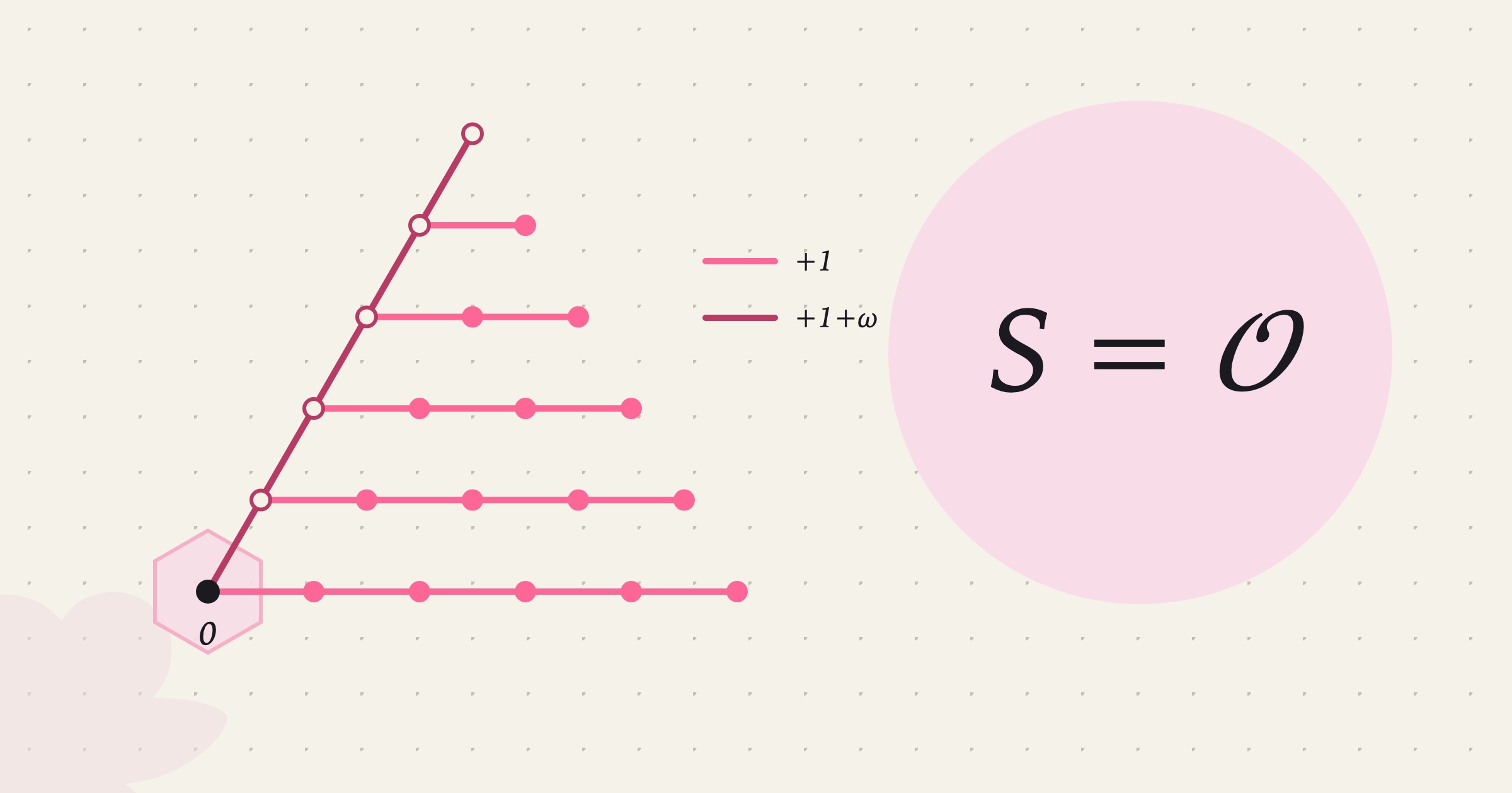
The canonical representatives form a hexagonal wedge in the Eisenstein lattice. We use a spanning tree whose edges differ by either  or
or  . Accumulating subtree sums along those two edge classes reduces the weighted sum to

For  coefficient buckets, the reducer uses exactly
  group additions, followed by one cheap endomorphism.
The bucket contents themselves are reduced with the batch-affine machinery already used elsewhere in our code. Independent affine additions at one tree level share a field inversion. The final bucket sums are then integrated by the hexagonal reducer. Bucket reduction is the dominant phase, roughly three quarters of the zero-check time.
The resulting backend is competitive as an ordinary arbitrary-base MSM.
The planner must look at scalar magnitudes
A planner chooses between the orbit backend and the existing Signed-Booth GLV backend, and the number of terms alone cannot predict their costs: prover MSMs are full of boolean columns, byte-sized values, and zero padding, and the joint Eisenstein representation uses more, narrower windows than Booth. The planner therefore decomposes the scalars first, records how many GLV components and joint scalars reach each bit position, and counts only the windows and assignments each backend would actually process.
Fixed bases make more multipliers reusable
The six units are cheap even without preparation. Fixed bases let us make a much larger set of Eisenstein multipliers cheap by computing their point images once.
Choose a set of multipliers  and retain

for every fixed base  . A radix digit can then factor as

where:
 is a free coordinate rotation and sign;
- selects one prepared point;
- selects a coefficient bucket.
The online contribution is

The extra multiplier does not add a curve operation to the check. It changes which prepared affine point is loaded.
The default codebook uses  and the subgroup

inside the unit group of  . Here

and

This produces:
- 256 prepared variants per fixed base;
- 32 coefficient buckets per window;
- 19 main windows for the approximately 127-bit GLV components.
For comparison, quotienting a width-7 Eisenstein window only by the six units would require 2,731 coefficient buckets. That width is not useful without preparation.
Each prepared point stores  , or 96 bytes. At roughly 2,000 fixed bases and 256 variants, the table occupies about 48 MiB. This buys more than a generic time-memory tradeoff: one prepared point stands in for an entire residue class under the CM action.
The degree-3 and degree-7 maps
The elements  and
and  are not additional geometric automorphisms of Vesta. They are non-unit complex-multiplication endomorphisms whose degrees equal their Eisenstein norms.
For a  curve
curve

let  . The degree-3 endomorphism
  has the affine formula

During preparation, these maps are batch-evaluated with shared inversions to scan the supplied bases for relations. The implementation computes the images in one batch, then computes

with a second batch-affine addition pass that reuses the images.
The hot zero-check loop does not evaluate a degree-3 or degree-7 isogeny for every digit. Their main role is algebraic: their residue classes generate useful sets of prepared multipliers. The online path selects already prepared images.
The relation scan looks for fixed bases related by ,  , and
, and  for ; a matched base is dropped from the prepared set and its scalar folded into its partner before recoding. This rarely helps independent random URS points, but it handles duplicates and protocol-defined symmetries without a separate path.
Alpha-only codebooks have a particularly simple table construction: their exact lifts are odd multiples of either or , so the table is built with two batched odd-multiple chains, one from  and one from
  . Other codebooks, including the default, evaluate their multipliers with the existing shared GLV batch ladder.
Residue factorization is not enough
The prepared point is the exact point

It is therefore not sufficient for a digit to be congruent to  modulo
  . The scalar recurrence must subtract the same exact Eisenstein integer whose point image is being used.
For every residue, the codebook chooses exact integer lifts and stores the carry induced by

The recurrence is

The codebook constructor independently derives and checks:
- the residue subgroup and its closure;
- the
 -cosets used as prepared variants;
 - the orbits used as coefficient buckets;
- the exact integer lift of every variant and coefficient;
- coverage of every nonzero residue;
- the exact carry for every table entry.
The prepared digit set is not a canonical number system, so repeated recoding is not required to terminate at zero. We run a fixed number  of main windows and retain a small residual
  :
:

The residuals are evaluated with the unprepared Eisenstein-orbit backend. Their size is bounded when the codebook is constructed and asserted after every recoding.
The prepared table is built in process from the supplied bases and is not serialized. A corrupted prepared table would change the equation being checked, so deserialization would require a separate table-validation and binding design.
The coefficient program is fixed too
Once the main buckets have been reduced, the implementation still needs

The coefficients  are fixed by the codebook. We therefore generate a static program for them.
Each coefficient is recoded in radix two with digits from  . A nonzero digit means adding a unit rotation of the corresponding bucket sum. A 0-1 shortest-path search finds a minimum-weight recoding for every coefficient, and the orbit representative search prefers coefficients with lower program weight.
A large program is stored by binary position: all operands at one position are reduced together with the batch-affine tree, then a short Horner pass combines the position sums. This is only profitable for large programs; small ones run instead as straight-line projective mixed additions.
Dynamic commitments should not widen the residual tail
Before this work, the verifier evaluated the whole equation with one tuned GLV MSM. The prepared path splits it: the fixed-base portion runs prepared, and every remaining point is still evaluated exactly once.
The URS bases are fixed, but a verifier equation also contains non-prepared commitment points, many of them proof-specific. These extra terms stay out of the residual tail. The fixed residuals are small and need only a few narrow windows; a single full-width extra scalar would force the tail through a complete scalar window schedule over every row, including all of the fixed bases, and would have to be multiplied by  , because the final Horner reconstruction multiplies the entire tail by
  .
.
The extras instead run as an independent MSM

alongside the prepared fixed-base part  , and the final check evaluates

Small extra counts run as a serial Signed-Booth MSM; larger ones go through the normal MSM planner. Under parallelism, the extras MSM runs concurrently with the main prepared windows and the fixed residual tail.
Splitting the equation gives up some of the amortization of one large MSM, so the prepared path stays profitable until the dynamic terms approach the fixed-base count; past that, a guard falls back to the combined MSM.
Results
The 2,048-term zero-check benchmark compares as follows on a 32-core x86-64 system with the portable field backend:
| implementation | 1 worker | 8 workers |
|---|---|---|
| current Signed-Booth MSM | 12.60 ms | 3.30 ms |
| prepared zero-check | 7.87 ms | 1.51 ms |
This is approximately a 1.60× speedup serially and 2.19× on eight workers. The benchmark's bases and scalars are synthetic, with planted relations that the preparation scan folds, so it measures the backend rather than the production verifier equation.
Dynamic terms stay cheap below the guard: 48 extras add about a millisecond to a check, and 512 add about 4 ms, the cost of an independent MSM of that size.
As an ordinary arbitrary-base MSM on uniformly full-width inputs, the Eisenstein-orbit backend measured a few percent faster than Booth serially and 30 to 65 percent faster on 32 workers, where its many narrower windows expose more parallel work.
End to end, validating a one-Action Ironwood bundle, signatures and transcript work included, compares as follows:
| configuration | 1 worker | 8 workers |
|---|---|---|
| before this work | 18.68 ms | 4.62 ms |
| this work, unprepared | 16.53 ms | 4.48 ms |
| this work, prepared | 13.21 ms | 3.65 ms |
The figures are medians across alternated runs on the same system, with preparation done before the timed calls. With the fixed bases prepared, validation takes 29% less time on one worker and 21% less on eight. The unprepared row shows the new MSM stack on its own: about 12% less serial time, and parity within measurement noise on eight workers.